L2: Multiplying and Factoring#
Eigenvectors#
Eigenvectors are vectors that do not change direction when you change the basis by a matrix \(A\). Following is an animation example.
Thus, it’s easy to understand that the eigenvalues are the scale factors of the eigenvectors. In following case, the vector \([-1\ 1]^T\) has been stretched into two times of its original length. So the eigenvelue is \(2\).
Show code cell source
from IPython.display import Image
Image('./imgs/l2-eigenvector.gif')
Important
Thus, the eigenvectors capture the esstenial information of the matrix \(A\), i.e., capture the unchanged direction of the matrix \(A\). Now let’s look at the famous equation \(Av=\lambda v\) where \(v\) is the eigenvector of \(A\) and \(\lambda\) is the eigenvalue of \(A\).
Why does this equation hold? Recall the multilpication of \(Av\) indicates we have a vector \(v\) in our coordinate system and we translate it into Jeniffer’s coordinate system with \(A\). Since the eigenvector \(v\) does not change its direction and only scale its length, the result of \(Av\) equals to scale \(v\) with \(\lambda\). Thus, the equation \(Av=\lambda v\) holds.
Some math trick for eigenvectors#
Since we that if the product of a matrix and a vector is zero, either the vector is zero or the columns of the matrix is not totoally independent. Which means the matrix is not full rank. Thus, the \(det(A-\lambda I)=0\).
Eigenvector may not exist. This can be understand in two ways: 1) when you rorate the coordinate system, all of the vector has been changed its direction. Thus, no eigenvector. 2) When \(det(A-\lambda I)\neq0,\forall \lambda\), then \(v\) must be zero vector. When eigenvector does not exist, either does the eigenvalue.
One eigenvalue may correspond to multiple eigenvectors. Imagine you just zoom in the coordinate system by 2 times. Then the eigenvalue is 2 but the corresponding eigenvector is the vectors on both axises.
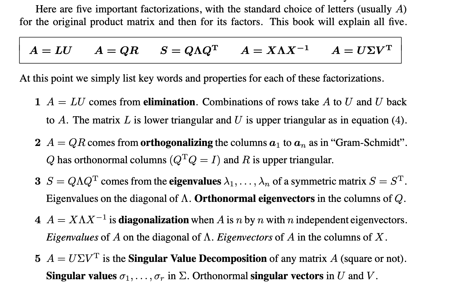
Another famous equation called digonalization: \(X^{-1}AX=\Lambda\) where columns of \(X\) is the eigenvectors of \(A\) and \(\Lambda\) is the diagonal matrix whose diagonal elements are the eigenvalues of \(A\). Why it holds? Firstly, we have \(AX=\lambda X\) according to the definition of eigenvector. Then we have \(X^{-1}AX=X^{-1}\lambda X=\lambda I=\Lambda\). If you leave \(A\) on the left, you will have \(A=X\Lambda X\) which is exactly the \(4\)-th equation introducted above in the book.
Conclusion 1#
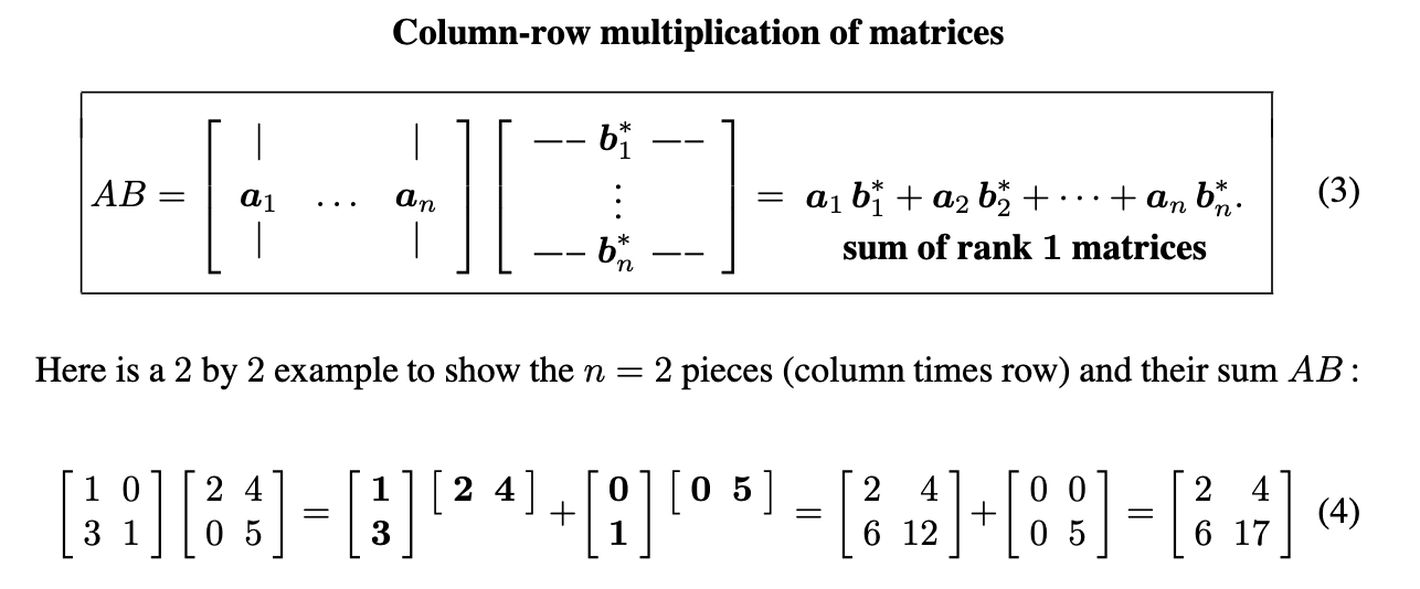
The multiplication of two matrices can be considered as \(n\) columns vectors multiplies \(n\) row vectors.
Show code cell source
from IPython.display import Image
Image('./imgs/l2-matrix-multiplication.png')
Conclusion 2#
The multiplication time of two matrices whose size are \(m\) by \(n\) and \(n\) by \(p\) is \(O(mnp)\).
Factorization#
Show code cell source
from IPython.display import Image
Image('./imgs/l2-factorization.png')
Important
When we multiply a matrix by a vector, i.e., \(Ax\). It can be considered as an kind of translation. The matrix \(A\) describe the basis of the new coordinate system, and the vector \(x\) describe coordinate of the point in the new coordinate system. Thus, the product of \(Ax\) is actually get the coordinate of the vector \(x\) in the old coordinate system.
In the case we have a vector \(y\) in Jeniffer’s coordinate system, we want to rotate it with 90 degrees, what’s the resutl? As we know, when we rotate our coordinate system, the basis will transformed from \(\left[\begin{array}{ll}1&0 \\ 0 &1\end{array}\right]\rightarrow\left[\begin{array}{ll}0&-1 \\ 0&1\end{array}\right]=A\). But this is the roration transformation in our coordinate system. To apply it to Jeniffer’s coordinate system, we have to translate the vector \(y\) to our coordinate system firstly, i.e., \(y'=My\), where the columns of \(M\) represents the basis of Jeniffer’s coordinate system in our coordinate system. Then we apply the rotation transformation \(A\) to the vector \(y'\), i.e., \(y''=Ay'=AMy\). Finally, we translate the vector \(y''\) back to Jeniffer’s coordinate system, i.e., \(y'''=M^{-1}y''=M^{-1}AMy\).
So, when we look at some thing like \(M^{-1}AM\), we know it is trying to do a transformation in Jeniffer’s coordinate system, but the transformation \(A\) is described in our sysmtem.
Reason the factorization holds#
For equation 4, as I explained before, \(AX=X\Lambda\rightarrow A=X\Lambda X^{-1}\), as long as \(A\) is a \(n\) by \(n\) matrix with \(n\) independent columns.
In case the matrix \(A\) meets some special conditions, i.e., it is not only a square matrix with \(n\) independent columns, but also a symmetric matrix, the eigenvectors will be orthogonal to each other. This can be proved easily but I don’t know why it holds geometically.
Moreover, if you normalize the length of eigenvectors to 1, then we have \(XX^T=I\rightarrow X^T=X^{-1}\). Now we have the equation 3, i.e., \(A=X\Lambda X^{-1}\rightarrow A=X\Lambda X^{T}\). The pros of this equation is that once we get the normalized eigenvectors, we avoide the trouble of computing its inverse matrix.
Columns space of \(AB\) is \(\leq\) column space of \(A\)#
Columns space of \(A\) is spaned by the independent columns in \(A\). The multiplication of \(AB\) is just a linear combination of these independent columns, which will not create new independent columns. Thus, the column space of \(AB\) is same or smaller than the column space of \(A\).