L3: Orthogonal Matrices#
Conclusion1: orthogonal subspace#
All the vectors in two different orthogonal subspaces are orthogonal to each other. Especially, the row space is orthogonal to null space.
We can find a fact that the vector \(x\) is orthogonal to every row of the matrix \(A\). Since the rows of the matrix forms the row space, and the columns of \(x\) forms the null space (in fact, we define all of the \(x\) statisfies this equation forms a null space). Thus, we know the row space is orthogonal to the null space.
Now, we have another interesting intuition about the \(Ax=0\). If the \(A\) is full rank, which means all of the rows are independent, assuming there are \(m\) rows, \(n\) columns, and \(m\leq n\), then we can not find a vector in \(\mathbb{R}^m\) that is perpendicular to the row space (since it full of the space \(\mathbb{R}^m\)). Thus, the number of independent vectors of \(x\) that satisfies the equation equals to the \(m-rank(A)\)
Understanding some geometric meaning of matrix#
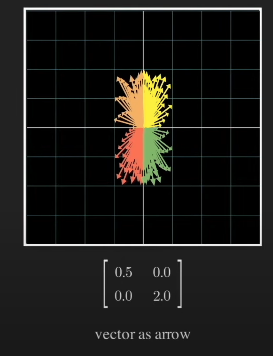
Digonal matrix is streching each axis since it only changes the sclae of each axis.
Show code cell source
from IPython.display import Image
Image('./imgs/l3-m1.png', retina=True)
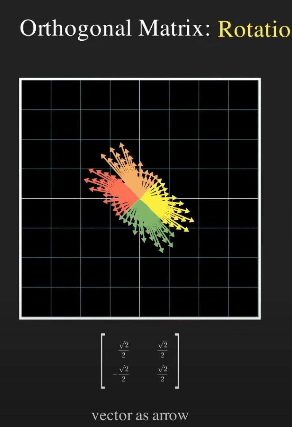
Orthogonal matrix is rotation since the length of each basis is not changing.
Show code cell source
from IPython.display import Image
Image('imgs/l3-m2.png', width=300)
Fun fact#
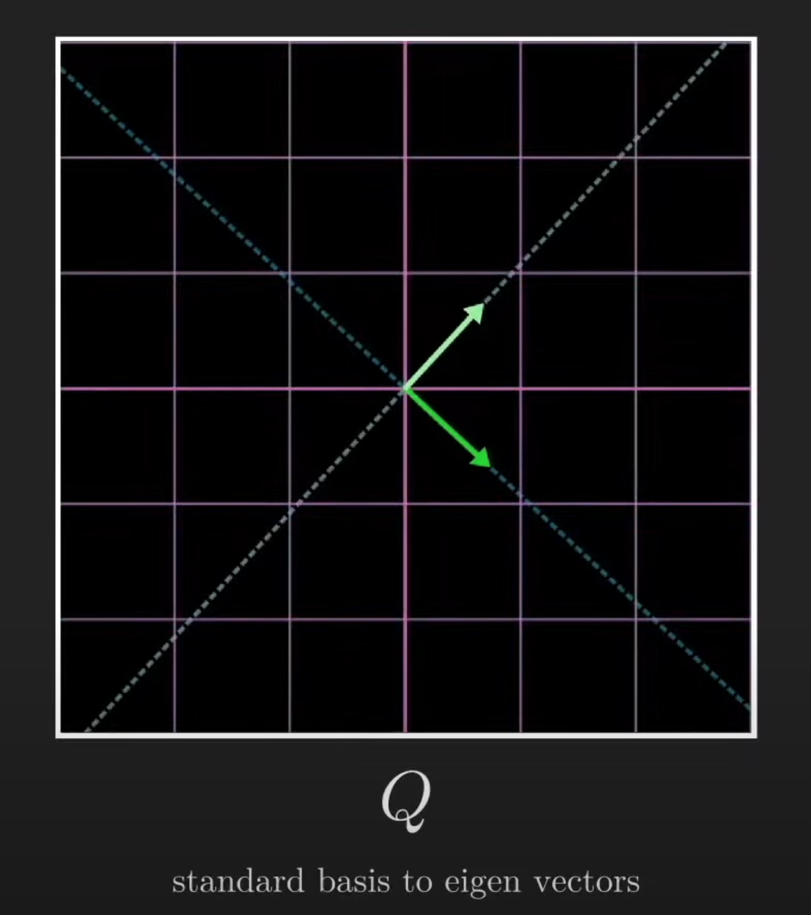
For an orthogonal matrix \(Q\), its inverse \(Q^-{-1}=Q^T\). If a matrix \(A\) is symmetric, then its eigenvectors form an orthogonal matrix. Then, the interesting thing happens. First of all, \(A\) can be considered as a transformation when you strech the space one the directions of eigenvectors. Then, since the eigenvectors are perpendicular to each other, the result of \(A\) can also be achieved by rotating the original axis since the eigenvectors are perpendicular and thus can be considered as the new axis.
Show code cell source
from IPython.display import Image
Image('imgs/l3-m3.png', retina=True)
Important
Thus, \(S=Q\Lambda Q^T\) can be understand as: any symmtric matrix can be considered as a tramsformation of three steps:
Rotate the axis by \(Q^T\), it transform the vectors in old coordinate to new coordinate.
Stretch the axis by \(\Lambda\), it streches the new axis by the eigenvalues.
Rotate the axis backward by \(Q\), it transform the vectors in new coordinate to old coordinate.
This is awesome, it means some complicated transformation can be achieved by several simple rotation and streching. Specifically, the conditions of such transformation is:
The sum of the dimensions of its eigenspaces is equal to the dimension \(n\) of the space. And the matrix is symmetric.
What’s the meaning of the first condition? I my understanding, it is same as we have \(n\) independent eigenvectors. But chatgpt does not agree with that. But I still did not understand it completely.
If the matrix is not symmetric but still holds the first part of above condition. We can decomposite the matrix into a less beautiful way, i.e., \(S=X\Lambda X^{-1}\), where columns of \(X\) are eigenvectors.
Decomposition with less condition#
First, let’s have a look a rectangle matrix with the size of \(2\times 3\).
Show code cell source
from IPython.display import Image
Image('imgs/l3-m4.png', retina=True)
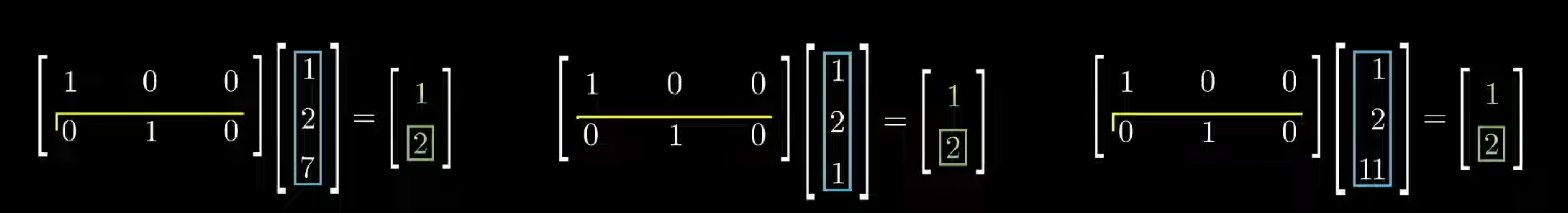
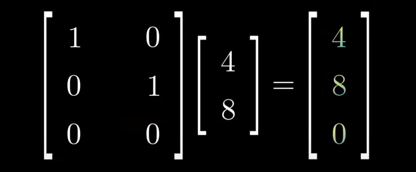
You can see, the dimension of the vector has been reduced from \(3\) to \(2\). Where the heck does the third dimension go? In fact the value of the third dimension contributes to the value of result vector. It does not just disappered, instead, the information of third dimension has been contained in the two dimension of the result vector. Although, in this picture, the dimension eraser assigns zero to the third dimension, which means it just discard the third dimension.
Show code cell source
from IPython.display import Image
Image('imgs/l3-m5.png', retina=True)
What happens when we apply an dimension adder? Where does the third dimension come from? If fact, the third dimension of reuslt vector is the reweighted sum of first two dimensions of the original vector (in fact it only has two dimensions). Although, in this picture, the dimension adder assigns zero to the first two dimensions.
SVD: singular value decomposition#
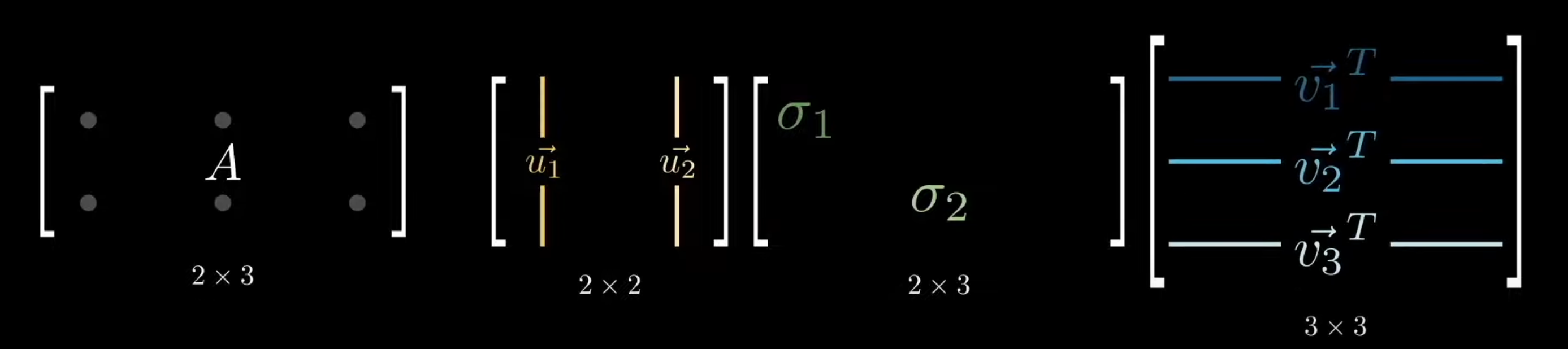
Recall the definition of the digonalization, where \(S=Q\Lambda Q^T\). The columns of \(Q\) are the eigenvectors of \(S\). But how can we get the eigenvectors from a rectangle matrix \(S\)? An amazing way is to get eigenvectors from the symmetric matrix \(SS^T\). Thus, the columns of \(Q\) are the eigenvectors of \(SS^T\).
What the \(Q^T\) corresponing to in this case? It is the eigenvectors of \(S^TS\). Thus, the columns of \(Q^T\) are the eigenvectors of \(S^TS\).
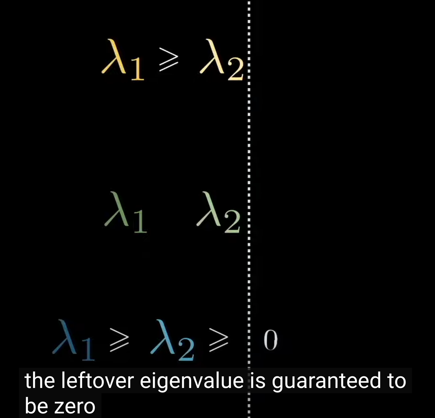
What’s the \(\Lambda\) corresponding to in this case? We don’t have eigenvalues for a rectangle matrix, but we can have singular values for them. In fact, it’s the eigenvalues of \(SS^T\) and \(S^TS\) sorted in the descending order (largest eigenvalues for these two matrices are same, rest of eigenvalues are zero, see following pictures). Thus, the diagonal of \(\Lambda\) are the singular values of \(S\).
Show code cell source
from IPython.display import Image
Image('imgs/l3-m6.png', width=800)
Show code cell source
Image('imgs/l3-m7.png', width=300)
Important
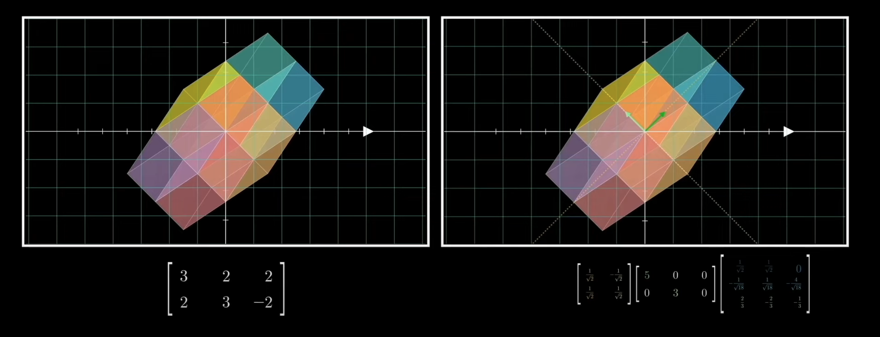
Thus, the SVD of \(S=U\sum V^*\) can also be considered as a sequence of simple transformation:
Rotate with \(V^*\).
Stretch with \(\sum\).
Rotate with \(U\).
The only thing different between SVD and digonalization is SVD might raise or reduce the dimension of the vector. :::
from IPython.display import Image
Image('imgs/l3-m8.png', width=800)
Interesting problem: projected vector#
Given a vector \(x\), we want to project it to another line, assume there is a vector \(v\) that is on the line. What’s the result of projection?
First, normalize the \(v\) to be \(u=v/||v||\). Then the length of the projection of \(x\) to the line is \(u^T\cdot x\). Finally, the prjection vector is \(u \cdot u^T \cdot x\).